5 Steps of Data Analysis By Using Microsoft Excel

Data analyst is an essential tool that enables organizations to gain deeper insights into their data. Utilizing Microsoft Excel for efficient data processing facilitates accurate and prompt decision-making while identifying trends and uncovering new business opportunities.

Table of content

1. The 5 steps for analyzing the sales_data_analysis.xlsx file in Microsoft Excel 365 are as follows
   1. Upload a document using the free online version of Microsoft Office 365
   2. Perform data analysis using sorting and filter tools.
   3. Perform data mining using the IF Function
   4. Create references between tables and search for information with VLOOKUP
   5. Perform data analysis using Pivot Table
      1. Pivot table

• Excel can help data analysis

• Excel work with a prepared spreadsheet that contains sale

The 5 steps for analyzing the sales_data_analysis.xlsx file in Microsoft Excel 365 are as follows

Upload a document using the free online version of Microsoft Office 365

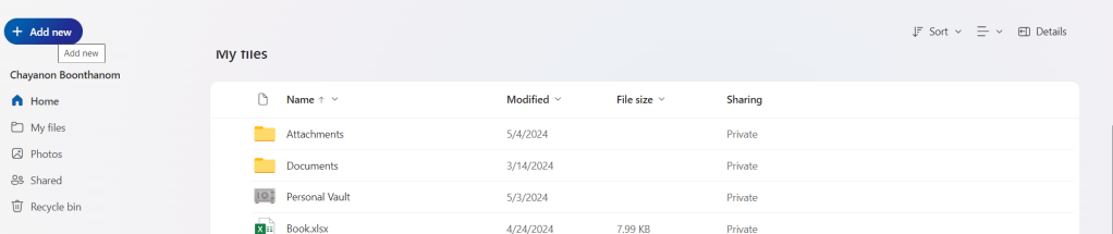
Click add new → File upload → then upload → sales_data_analysis_23.10.2024

• Go to Insert → Table to create a table that uses the header in the first column to filter data. → Click OK.

• To Create a table to filter data, see the picture below.

• Then filter the data shown in the picture below.

Set it up so that when you scroll down to view data in the rows below, the first column remains visible. This makes it much easier to reference the headings.

Perform data analysis using sorting and filter tools.

Which column should be prioritized for sorting data to make it more effective?

representative header and then select sort A to Z to sort it in alphabetical order

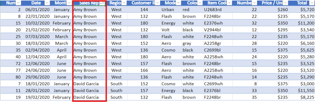
• after click it has been rearrange by alphabetical Sales Rep
• then to make it back to select sort in column date again
• can sort the Region by North.

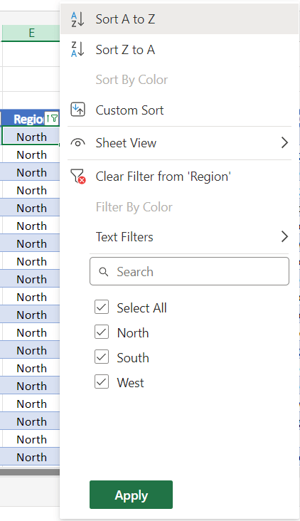
• To remove the filter, click the ‘Select All‘ checkbox to display sales from the North, South, and West regions, and then click.
• Then filter the Sales Rep column by the name David Garcia.

• you can see aggregate value in the bottom right corner.

This is how to use the sorting and filtering tools to rearrange your data.

Perform data mining using the IF Function

• The idea behind data mining is to take the data you already have and create new or additional data from it.
• The IF function is frequently used.

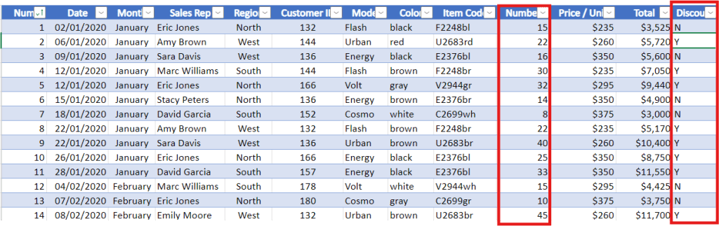
Samples show that when an order includes 20 chairs or more, the client receives a 5% wholesale discount.

Code for column Discount

=IF(J5>=20,"Y","N")

• Final Price column

Code for column Final Price

=IF(J5>20,0.95*L5,L5)

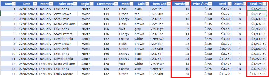
• column of Discount with Y is number ≥ 20 price is discount 5% final is 95% from total column
• column of Discount with N is number ≤ 20 price is same as the total

Create references between tables and search for information with VLOOKUP

Goal is to insert the company name using the client ID.

1. Create column Company Name between Customer ID and Color
2. Create column Company Name Representative between Company name and model

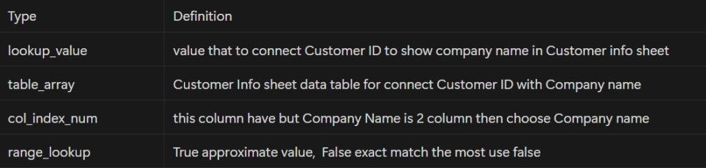
The explanation of the variables used in VLOOKUP.

VLOOKUP(lookup_value, table_aray, col_index_num, [range_lookup])

Create Company name column

=VLOOKUP(F5,'Customer Info'!$A$4:$C$12,2,FALSE)

Create Company name representative

=VLOOKUP(F5,'Customer Info'!$A$4:$C$12,3,FALSE)

to connect data between sales data and customer info sheet

can adding a dollar sign in front A4 and C12 to make data not change

Perform data analysis using Pivot Table

Method to start

• Typing control A and it will automatically highlight all the data in the table
• Then insert ———> Pivot table ———> click okay

• Recommend selecting new worksheet so it placement does not affect the other data that already exists

Pivot table

• define categories as either filters, columns, rows, value

• 1. drag Final Price to Value of pivot table
• 2. drag Sales Rep to columns of pivot table
• 3. drag Month to row of pivot table

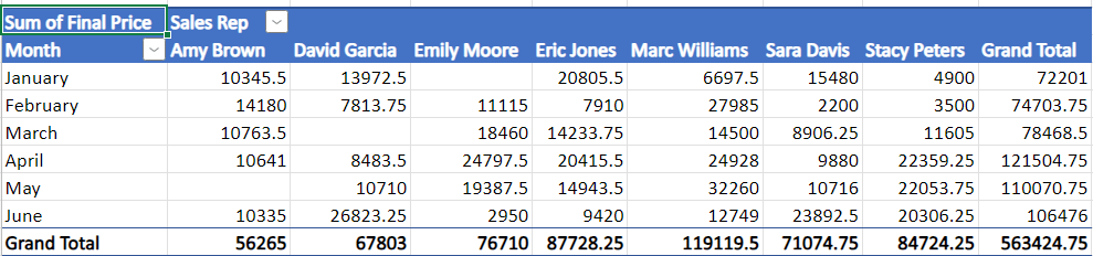
how many chairs of each model were sold in each month?

• Finally you have learned how to create pivot tables to summarize and look at comparisons within your data.

Access full Microsoft excel through below link:

Coursera Project Network Certificate

https://www.coursera.org/account/accomplishments/verify/2F13S7V2LEZF

Summary

Data analysts help organizations gain valuable insights from data. Using Microsoft Excel enhances decision-making by processing data efficiently and identifying trends and opportunities.